Investigation of some probabilistic properties of the Langford pairing problem
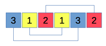
In combinatorial mathematics, a Langford pairing, also called a Langford sequence, is a permutation of the sequence of 2n numbers (1, 1, 2, 2, ..., n, n) in which the two ones are one unit apart, the two twos are two units apart, and more generally the two copies of each number k are k units apart. Langford pairings are named after C. Dudley Langford, who posed the problem of constructing them in 1958.
When does the Langford pairing exist?
Let’s consider an arrangement of n pairs of natural numbers within a sequence of length 2n, which satisfies conditions of the problem. Is it possible to obtain a Langford sequence for all values of n?
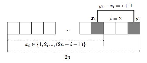
Every number i can be associated with two numbers: xi and yi, which represent the indices of the first and the second occurrence of the number in the sequence. Hence, according to the requirements of the problem, we can define the system of following constraints:
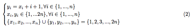
The third and the second constraints mean, that all values of xi and yi must be unique. Having the third constraint in mind, let’s calculate the sum of all xi and yi:
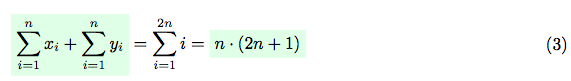
On the other hand, having the first constraint in mind, the sum of all xi and yi can be represented in a following way:

Hence, from equations (3) and (4) we have:
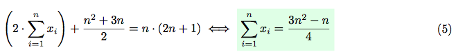
As far as the sum of all xi is integer, then  must be integer as well.
It is possible iff
must be integer as well.
It is possible iff 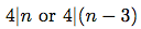 .
.
Hence, in case if the n pairs of natural numbers can be arranged into the sequence of
length 2n (with respect to the constraints of the problem).
Langford pairing and the random permutations
Let’s explore the possibility to obtain a Langford sequence (which will satisfy all constraints from equation (2)) as a result of the random permutation of the sequence of n pairs of natural numbers.
Expectation of the amount of correct placements
Let’s consider a discrete valued random variable  , which represents an amount of correct placements of pairs of numbers (which satisfy the first constraint from the system of constraints (2)).
In order to proceed, let’s represent as a sum of indicator random variables:

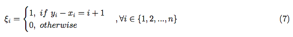
where  is an indicator random variable,
which indicates - whether the pair of i-th numbers placed correctly (with respect to the constraints from equation (2)):
is an indicator random variable,
which indicates - whether the pair of i-th numbers placed correctly (with respect to the constraints from equation (2)):
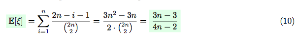
Due to the linearity of the expectation:
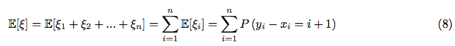
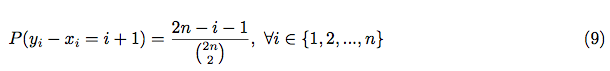
Where: 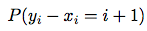 is a probability, that xi and yi are placed correctly (according to the constraints from equation (2)).
Let's calculate .
For every pair of numbers with index 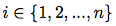 out of
  possible positions for xi and yi - there are only (2n − i − 1) positions, which satisfy constraints from equation (2).
For example:
possible positions for xi and yi - there are only (2n − i − 1) positions, which satisfy constraints from equation (2).
For example:
Hence:
So, expectation of the amount of correct placements can be represented as:
Variance of the amount of correct placements
Let’s calculate the variance of .
By definition of the variance, and according to the equation (6):
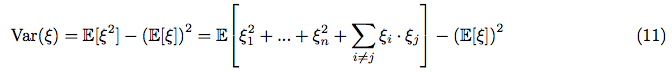
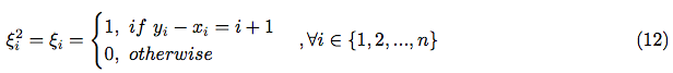
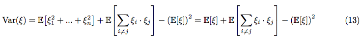
As far, as is an indicator random variable, then:
We can make use of the linearity property of expectation again:
However, we need to calculate somehow the value of: 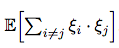 .
.
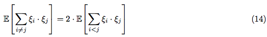
Due to the symmetry, we can consider only the cases, when i < j:
It turns out, that  is also an indicator random variable, which is defined in a following way:

Hence, we have:
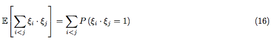
 is equal to a joint probability
 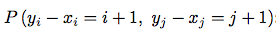 :
:

Where:
 - number of ways to place correctly the i-th and j-th pairs of numbers
 - number of ways to choose values for: xi, yi, xj and yj
Let’s calculate .
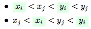
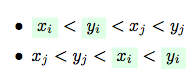
The set of all correct relative arrangements of xi, yi, xj and yj can be divided into three disjoint sets with interleaved ( ), nested (
 ) and separate (
 ) relative placements.
Hence:
) relative placements.
Hence:

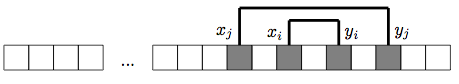
Interleaved arrangements:
Without loss of generality let’s consider only a first variant: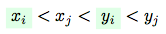 (the counting for the second variant will be exactly the same - so, we will just multiple an obtained result by 2).
In order to produce the correct interleaved placement, we need to choose the proper positions of the leftmost and rightmost occupied cells (xi and yj), and afterwards we can solely define the positions of yi and xj inside:
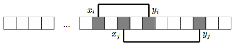
An amount of cells between the leftmost and rightmost occupied cells is:

where: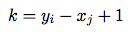
As far as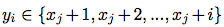 , then
 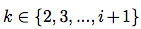 .
Hence the total amount of all possible interleaved placements is:
.
Hence the total amount of all possible interleaved placements is:
Nested arrangement:
In order to produce the correct nested placement, we need to choose the proper positions of the leftmost and rightmost occupied cells (xj and yj), and afterwards we should choose the proper positions for xi and yi inside:
An amount of ways to choose the proper positions for xj and yj is: (2n − j − 1). Now, we need to choose the proper positions for xi and yi inside, and an amount of ways to do so is: (j − i − 1).
Hence:

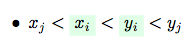
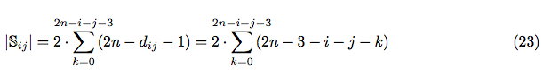
Separate arrangements:
Without loss of generality let’s consider only a first variant: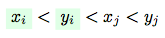 (the counting for the second variant will be exactly the same - so, we will just multiple an obtained result by 2).
In order to produce the correct interleaved placement, we need to choose the proper positions of the leftmost and rightmost occupied cells (xi and yj), and afterwards we can solely define the positions of yi and xj inside:
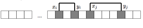
An amount of cells between the leftmost and rightmost occupied cells is:

where: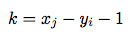
As far as , then
 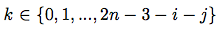 .
.
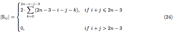
Hence, the total amount of all possible separate placements is:
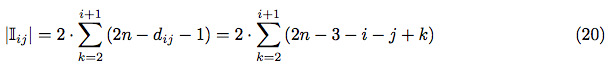
The tidy analysis shows, that in case if i + j > 2n − 3 any separate arrangement of i-th and j-th pairs of characters is impossible within 2n slots. Hence, the complete formula for || is:
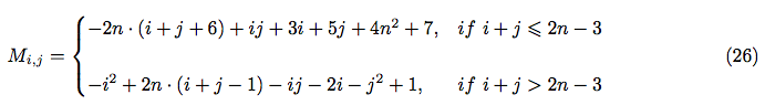
So, finally, using equations (20), (21) and (24) - we can express in terms of i, j and n:
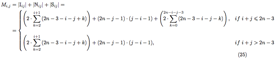
After simplification, we can obtain the closed form for :
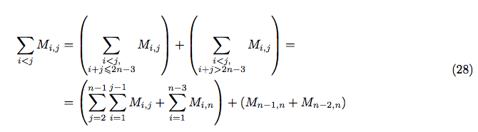
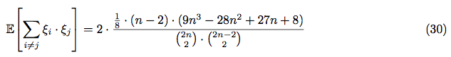
Now, we are almost ready to calculate 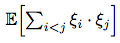 , using equations (16) and (17):
In order to calculate the sum  let’s consider separately the cases where
  and
and  :
:
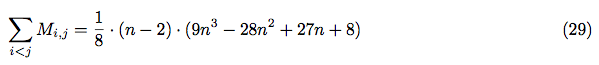
After simplification, we can obtain the closed form:
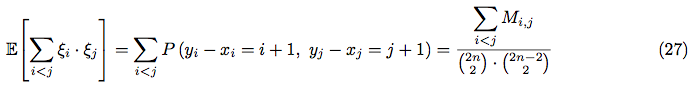
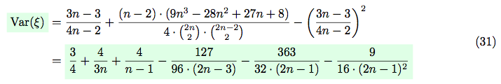
According to equations (14), (27) and (29) we can obtain the value of 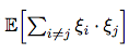 :
:
So, using equations (10), (13) and (14) we can calculate the variance:
Experimental evaluation
In order to verify derived formulas for expectation and variance, I have developed an application for simulation of random permutations on the sequences with different amounts of pairs of natural numbers. For every n application simulates 500000 random permutations, and calculates the average amount (and variance) of correctly placed pairs of numbers.
Below is presented the code of a Java application for simulation:
import java.util.*;

public class ExpectationVarianceCheck {

    public static void main(String[] args) {
        Random rnd = new Random(1);
        for (int size = 2; size < 46; size++) {
            evaluate(size, rnd);
        }
    }

    private static void evaluate(int size, Random rnd) {

        int trials_count = 500000;

        int correct_placements_cnt = 0;
        int correct_placements_cnt_sqr = 0;
        for (int i = 0; i < trials_count; i++) {
            List<Integer> characters = random_placement(size, rnd);
            int correct = calc_correct_placements(characters);
            correct_placements_cnt += correct;
            correct_placements_cnt_sqr += correct * correct;
        }

        double avg_correct_placements =
                (double) correct_placements_cnt / trials_count;
        double experimental_variance =
                (double) correct_placements_cnt_sqr / trials_count
                        - Math.pow(avg_correct_placements, 2);

        System.out.printf("%d  %3.3f  %3.3f  %3.3f  %3.3f %n",
                size, avg_correct_placements, expectation(size),
                experimental_variance, variance(size));
    }

    private static double expectation(int n) {
        return (3.0 * n - 3) / (4 * n - 2);
    }

    private static double variance(int n) {
        return 3.0 / 4 + 4.0 / (n - 1) + 4.0 / (3 * n)
                - 127.0 / (96 * (2 * n - 3)) - 363.0 / (32 * (2 * n - 1))
                - 9.0 / (16 * Math.pow(2 * n - 1, 2));
    }

    private static int calc_correct_placements(List<Integer> characters) {
        Map<Integer, Integer> first_occurrence = new HashMap<>();
        int correct = 0;
        for (int i = 0; i < characters.size(); i++) {
            int c = characters.get(i);
            if (first_occurrence.get(c) == null) {
                first_occurrence.put(c, i);
            } else {
                int firstOccurrencePos = first_occurrence.get(c);
                if (i - firstOccurrencePos - 1 == c) {
                    correct++;
                }
            }
        }
        return correct;
    }

    private static List<Integer> random_placement(int size, Random rnd) {
        List<Integer> characters = new ArrayList<>();
        for (int i = 1; i <= size; i++) {
            characters.add(i);
            characters.add(i);
        }
        Collections.shuffle(characters, rnd);
        return characters;
    }
}
Below is presented a table with comparison of the expectation and variance obtained experimentally and calculated, based on the derived formulas:
| n (amount of pairs of numbers) | average amount of correct placements | theoretical expectation | experimental variance | theoretical variance |
|---|---|---|---|---|
| 2 | 0.502 | 0.500 | 0.250 | 0.250 |
| 3 | 0.601 | 0.600 | 0.462 | 0.462 |
| 4 | 0.643 | 0.643 | 0.520 | 0.520 |
| 5 | 0.669 | 0.667 | 0.562 | 0.560 |
| 6 | 0.681 | 0.682 | 0.590 | 0.589 |
| 7 | 0.691 | 0.692 | 0.611 | 0.611 |
| 8 | 0.699 | 0.700 | 0.630 | 0.628 |
| 9 | 0.708 | 0.706 | 0.644 | 0.641 |
| 10 | 0.713 | 0.711 | 0.653 | 0.651 |
| 11 | 0.716 | 0.714 | 0.660 | 0.660 |
| 12 | 0.720 | 0.717 | 0.670 | 0.667 |
| 13 | 0.719 | 0.720 | 0.674 | 0.674 |
| 14 | 0.723 | 0.722 | 0.679 | 0.679 |
| 15 | 0.724 | 0.724 | 0.684 | 0.684 |
| 16 | 0.725 | 0.726 | 0.688 | 0.688 |
| 17 | 0.728 | 0.727 | 0.695 | 0.691 |
| 18 | 0.727 | 0.729 | 0.692 | 0.695 |
| 19 | 0.730 | 0.730 | 0.699 | 0.698 |
| 20 | 0.730 | 0.731 | 0.700 | 0.700 |
| 21 | 0.733 | 0.732 | 0.703 | 0.703 |
| 22 | 0.734 | 0.733 | 0.705 | 0.705 |
| 23 | 0.732 | 0.733 | 0.705 | 0.707 |
| 24 | 0.735 | 0.734 | 0.711 | 0.708 |
| 25 | 0.733 | 0.735 | 0.710 | 0.710 |
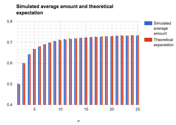
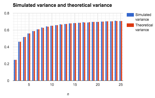
As you can see, the values obtained via derived formulas of expectation and variance are consistent to the values obtained via computer simulation.
Probabilistic bounds
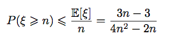
Having the explicit expressions for expectation and variance we can make use of a couple of probabilistic inequalities, in order to estimate the probability of obtaining the correct placement of all n pairs of numbers:
Markov's inequality:
Chebyshev's inequality:
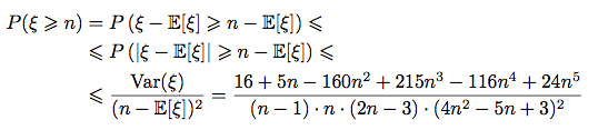
Unfortunately, these probabilistic bounds are still very weak.
Speculation around the Poisson distribution
Strictly speaking, the indicator random values of are not independent, hence generally speaking, we can’t model the distribution of values of using the Poisson distribution.
Nevertheless, let’s consider the values of expectation and variance for the large amounts of pairs n:
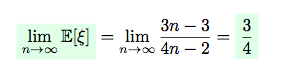

We can see, that 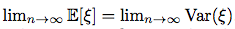 .
Hence, to some extent, I assume that it is still viable to use a Poisson distribution as a rough approximation of the distribution of values of the random variable .
This assumption is also based on the observation, that occurrence of the correctly placed pair of numbers is a rare event.
.
Hence, to some extent, I assume that it is still viable to use a Poisson distribution as a rough approximation of the distribution of values of the random variable .
This assumption is also based on the observation, that occurrence of the correctly placed pair of numbers is a rare event.
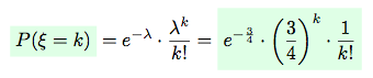
The event rate of the given Poisson distribution is  .
Hence, the probability of occurrence of k correctly placed pairs is:
.
Hence, the probability of occurrence of k correctly placed pairs is:
Let’s evaluate adequacy of the Poisson approximation experimentally (again, using the computer simulation):
import java.util.*  ;

public class PoissonDistributionCheck {

    public static void main(String[] args) {
        Random rnd = new Random(1);
        for (int size = 20; size < 41; size += 5) {
            evaluate(size, rnd);
            System.out.println();
        }
    }

    private static void evaluate(int size, Random rnd) {
        int trialsCount = 500000;
        Map<Integer, Integer> correct_placements_count = new TreeMap<>();
        for (int i = 0; i < trialsCount; i++) {
            List<Integer> characters = random_placement(size, rnd);
            int correct = calc_correct_placements(characters);
            int count = correct_placements_count.getOrDefault(correct, 0);
            correct_placements_count.put(correct, count + 1);
        }
        for (int correct : correct_placements_count.keySet()) {
            int simulated_count = correct_placements_count.get(correct);
            double simulated_prob = (double) simulated_count / trialsCount;
            System.out.printf("%d %d %1.5f %1.5f %n", size, correct, simulated_prob, poisson_prob(correct));
        }
    }

    private static double poisson_prob(int correct) {
        long fact = factorial(correct);
        return Math.exp(-0.75) * Math.pow(0.75, correct) / fact;
    }

    private static long factorial(int n) {
        long fact = 1;
        for (int i = 1; i <= n; i++) {
            fact *= i;
        }
        return fact;
    }

    private static int calc_correct_placements(List<Integer> characters) {
        Map<Integer, Integer> first_occurrence = new HashMap<>();
        int correct = 0;
        for (int i = 0; i < characters.size(); i++) {
            int c = characters.get(i);
            if (first_occurrence.get(c) == null) {
                first_occurrence.put(c, i);
            } else {
                int firstOccurrencePos = first_occurrence.get(c);
                if (i - firstOccurrencePos - 1 == c) {
                    correct++;
                }
            }
        }
        return correct;
    }

    private static List<Integer> random_placement(int size, Random rnd) {
        List<Integer> characters = new ArrayList<>();
        for (int i = 1; i <= size; i++) {
            characters.add(i);
            characters.add(i);
        }
        Collections.shuffle(characters, rnd);
        return characters;
    }
}
Below is presented an example of table (for n = 40) with comparison of observed distribution and the Poisson distribution:
| n | k | Observed distribution of the values of |
Poisson distribution |
|---|---|---|---|
| 40 | 0 | 0.47407 | 0.47237 |
| 40 | 1 | 0.35732 | 0.35427 |
| 40 | 2 | 0.13153 | 0.13285 |
| 40 | 3 | 0.03100 | 0.03321 |
| 40 | 4 | 0.00533 | 0.00623 |
| 40 | 5 | 0.00068 | 0.00093 |
| 40 | 6 | 0.00008 | 0.00012 |
| 40 | 7 | 0.00000 | 0.00001 |
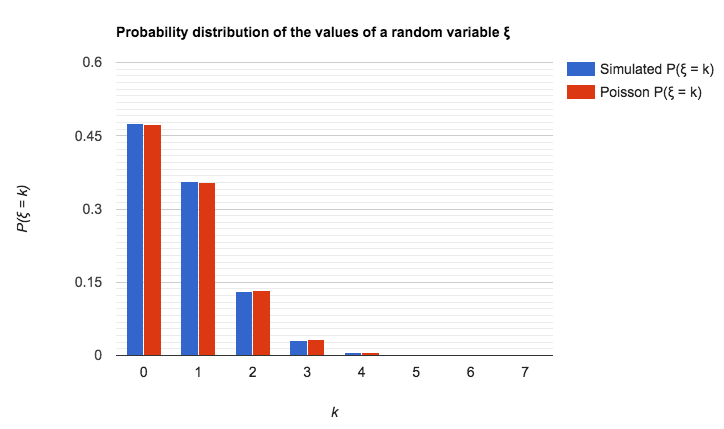
As you can see, the Poisson distribution can be used as an approximate upper bound of distribution of values of a random variable, which represents an amount of correctly placed pairs of numbers (after the random shuffling).